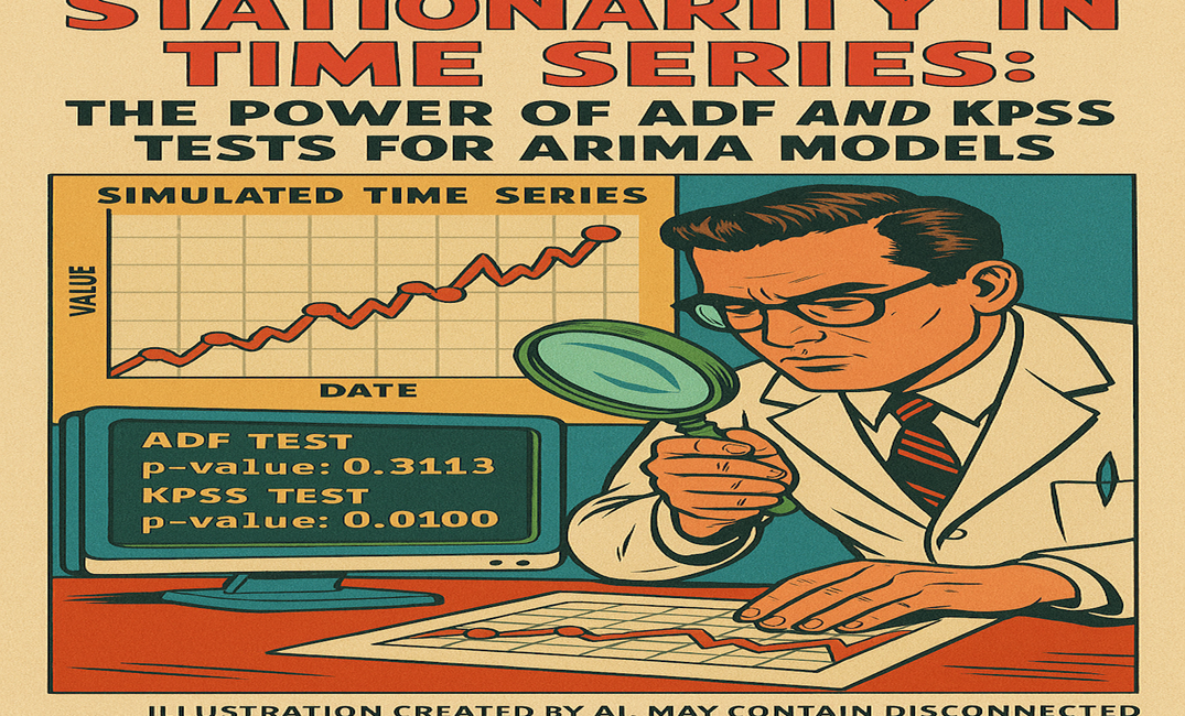
Stationarity in Time Series: The Power of ADF and KPSS Tests for ARIMA Models

By Izairton Vasconcelos
12 min read

Table of Contents

In time series analysis, understanding the structure of the data over time is a critical step before applying any predictive model.

Stationarity—that is, the statistical constancy of mean, variance, and autocorrelation—is the fundamental requirement to ensure the reliability of models in the ARIMA family.

Ignoring this condition can lead to biased, unstable, and practically useless forecasts. In this article, we explore how the ADF (Augmented Dickey-Fuller) and KPSS (Kwiatkowski-Phillips-Schmidt-Shin) tests complement each other to carry out this verification with statistical precision and technical rigor.


Why Use Stationarity Tests?

Models such as ARIMA and SARIMA operate under the assumption that the time series is stationary. If the series presents trend or non-constant variance over time, model parameters will not converge properly, and forecasts will become unstable. Stationarity tests offer a formal and mathematical diagnosis of this condition, allowing the analyst to apply transformations (like differencing or log transformation) only when necessary. Applying both tests—ADF and KPSS—provides a more complete reading, as they have opposite null hypotheses, functioning as complementary tools in the diagnosis.


Technical and Logical View of the ADF and KPSS Tests

The ADF test assumes as the null hypothesis that the series is not stationary, i.e., that it has a unit root. On the other hand, the KPSS test assumes the opposite: that the series is stationary. The cross-analysis of these two tests is especially useful to reduce uncertainty in the decision to apply transformations. If both point to the same conclusion, the level of confidence in the diagnosis increases. Additionally, including a plot of the series helps with visual interpretation, connecting formal statistics to analytical intuition.


Choosing the Right Approach: Visual vs. Statistical

Visually inspecting a time series can be useful to detect trends or seasonality, but this approach is highly subjective. In professional projects—especially involving finance, capital markets, or demand forecasting—decisions cannot rely on guesswork. Therefore, applying statistical tests becomes mandatory. Moreover, tests like ADF and KPSS can be easily integrated into automated pipelines, enabling reuse, traceability, and auditability—which are foundational pillars of any robust analytical workflow.


Real Example: Diagnosing Stationarity with a Simulated Series

For this study, we use a monthly simulated time series with non-stationary characteristics: an upward trend with accumulated random fluctuations over 36 periods. This type of series is common in scenarios such as inflation, commodity prices, or sales volume. The goal here is to replicate a realistic scenario of raw data still untreated, testing how ADF and KPSS behave when faced with a pattern that has a clear trend.


Full Python Script: Simulated Series + Stationarity Tests

To robustly assess the stationarity of a time series, it is essential that data generation, graphical visualization, and statistical tests are integrated into a single flow. This not only improves code organization but also ensures that the data being analyzed corresponds exactly to what is displayed in the charts and tested. Below is the complete script to generate the simulated series, plot the chart, and apply ADF and KPSS tests. This script can be run entirely in VSCode by saving it as testes_estacionaridade.py.

# test_stationary.py
# Author: Izairton Vasconcelos
# Purpose: Generate a non-stationary time series and apply ADF and KPSS tests
# Compatible with Python 3.8+ and tested in VSCode

import pandas as pd
import numpy as np
import matplotlib.pyplot as plt
from statsmodels.tsa.stattools import adfuller, kpss

def generate_simulated_series(seed=42, mean=2, std=3, size=36, initial_value=100):
    """
    Generate a non-stationary time series by applying cumulative sum to random noise.
    The result simulates a realistic upward trend (stochastic drift).
    
    Parameters:
        seed (int): Random seed for reproducibility
        mean (float): Mean of the normal distribution
        std (float): Standard deviation of the normal distribution
        size (int): Number of periods (months)
        initial_value (float): Starting point of the time series
    
    Returns:
        pd.Series: Time series indexed by monthly dates
    """
    np.random.seed(seed)
    dates = pd.date_range(start="2020-01-01", periods=size, freq="ME")
    values = np.cumsum(np.random.normal(loc=mean, scale=std, size=size)) + initial_value
    return pd.Series(values, index=dates)

def plot_series(ts, filename="stationarity_series.png"):
    """
    Plot the time series and save it as an image file.
    
    Parameters:
        ts (pd.Series): The time series to plot
        filename (str): Name of the output image file
    """
    print("📈 Displaying the time series chart...")
    plt.figure(figsize=(10, 4))
    plt.plot(ts, marker='o', color='blue')
    plt.title("🚦 Simulated Time Series")
    plt.xlabel("Date")
    plt.ylabel("Value")
    plt.grid(True)
    plt.tight_layout()
    plt.savefig(filename)
    plt.show()
    print(f"✅ Chart saved as: {filename}")

def run_adf_test(ts):
    """
    Apply the Augmented Dickey-Fuller test and print results.
    ADF H₀: the series is non-stationary.
    
    Parameters:
        ts (pd.Series): Time series to test
    """
    print("\n📌 ADF Test (Augmented Dickey-Fuller):")
    result = adfuller(ts)
    print(f"  Test Statistic: {result[0]:.4f}")
    print(f"  p-value:        {result[1]:.4f}")
    print("  => Reject H₀? ", "Yes ✅" if result[1] < 0.05 else "No ❌")

def run_kpss_test(ts):
    """
    Apply the KPSS test and print results.
    KPSS H₀: the series is stationary.
    
    Parameters:
        ts (pd.Series): Time series to test
    """
    print("\n📌 KPSS Test (Kwiatkowski-Phillips-Schmidt-Shin):")
    result = kpss(ts, regression="c", nlags="auto")
    print(f"  Test Statistic: {result[0]:.4f}")
    print(f"  p-value:        {result[1]:.4f}")
    print("  => Reject H₀? ", "Yes ❌" if result[1] < 0.05 else "No ✅")

def main():
    """
    Main function to execute the entire analysis:
    - Generate the time series
    - Plot the chart
    - Apply ADF and KPSS stationarity tests
    """
    print("🚀 Starting stationarity analysis...\n")
    
    # Step 1: Generate the simulated time series
    ts = generate_simulated_series()
    
    # Step 2: Visualize the series
    plot_series(ts)
    
    # Step 3: Apply the ADF test
    run_adf_test(ts)
    
    # Step 4: Apply the KPSS test
    run_kpss_test(ts)
    
    print("\n🏁 Analysis complete.")

# Standard Python boilerplate
if __name__ == "__main__":
    main()

This script covers the entire essential logic: trend simulation (via np.cumsum()), visualization using matplotlib, and statistical diagnosis with statsmodels. Using ADF and KPSS together allows a dual and precise reading of the series' behavior.


Generated Images: Visual Analysis and Statistical Interpretation

Chart: Time Series Visualization

The chart generated by the script displays the time series ts, simulated with an accumulative behavior over 36 monthly periods. The section responsible for generating and saving the chart is:

plt.figure(figsize=(10, 4))
plt.plot(ts, marker='o')
plt.title("🚦Simulated Time Series")
plt.xlabel("Date")
plt.ylabel("Value")
plt.grid(True)
plt.tight_layout()
plt.savefig("serie_estacionaridade.png")
plt.show()

What it shows:

The upward curve reflects the non-stationary nature of the series, generated by:

ts = pd.Series(np.cumsum(np.random.normal(loc=2, scale=3, size=36)) + 100, index=datas)

This cumulative pattern simulates a stochastic drift often found in real-world economic series — such as inflation, cumulative revenue, or account balances — where there is a persistent upward trend. The visualization shows fluctuations with increasing mean and variance over time, violating the fundamental principles required by ARIMA and SARIMA models.

Practical usefulness:

  • Provides an initial visual clue that the series is not stationary.
  • Justifies the application of formal stationarity tests.
  • Helps the analyst decide whether a transformation like .diff() is necessary to stabilize the series.
  • In business contexts, such a graph is also essential for communicating behavioral patterns to stakeholders in an accessible and objective way.

VSCode Terminal: Execution and Test Results

The complete script execution in the VSCode terminal confirms the expected behavior of the series and highlights the diagnostic power of the ADF and KPSS tests. The output shown was:

Teste ADF (Augmented Dickey-Fuller):

Estatística: -1.9447
p-valor: 0.3113
=> Rejeita H₀? Não❌

Teste KPSS (Kwiatkowski-Phillips-Schmidt-Shin):

Estatística: 0.7478
p-valor: 0.0100
=> Rejeita H₀? Sim❌

ADF Test – Augmented Dickey-Fuller

adf_result = adfuller(ts)

Purpose: Tests the null hypothesis that the series is not stationary (i.e., it has a unit root).

Output interpreted:

Test statistic = -1.9447
p-value = 0.3113 → p ≥ 0.05
Result: Fail to reject H₀ → The series is non-stationary❌

KPSS Test – Kwiatkowski-Phillips-Schmidt-Shin

kpss_result = kpss(ts, regression="c", nlags="auto")

Purpose: Tests the null hypothesis that the series is stationary.

Parameters used:

  • regression="c" → intercept only
  • nlags="auto" → automatically chosen lag number

Output interpreted:

Test statistic = 0.7478
p-value = 0.0100 → p < 0.05
Result: Reject H₀ → The series is non-stationary❌

⚠️ The script also returned an InterpolationWarning, indicating that the statistic's value is outside the p-value lookup table. However, the diagnosis remains valid: the p-value is low enough to reject the null hypothesis of stationarity.

Integrated logic summary:

Test

Null Hypothesis (H₀)

Desired Result (p < 0.05)

Actual Diagnosis

ADF

Series is not stationary

Reject H₀ → Stationary

❌ Not rejected

KPSS

Series is stationary

Reject H₀ → Non-stationary

✅ Rejected

Practical conclusion:
Since ADF fails to reject H₀ and KPSS rejects H₀, we have a clear and coherent diagnosis: the series is non-stationary and should be transformed before modeling, preferably using ts.diff().

The Turning Point of the Analysis: When the Series Reveals Its Nature

If we were to pinpoint the exact line where Python “reveals the soul” of the time series — the moment where its statistical behavior becomes undeniable both in the terminal and in the plot — it would be this one:

ts = pd.Series(np.cumsum(np.random.normal(loc=2, scale=3, size=36)) + 100, index=datas)

Why is this line so special?

This is where the analytical breakthrough happens. The np.cumsum() function accumulates values from a normal distribution, simulating a stochastic drift — a progressive shift that distorts the mean of the series over time. This simple operation turns white noise (which would be stationary) into a sequence with a structural trend, a critical feature for illustrating non-stationarity.

Visually, this results in:

  • A chart that does not oscillate around a constant mean
  • A steadily increasing trajectory that never returns to the origin
  • A realistic pattern of continuous growth — like cumulative profits, inflation, compound interest, or population growth

Statistically, this very line of code lays the groundwork for the ADF and KPSS tests to detect — and confirm — that the series violates stationarity conditions.

Didactic insight:

💡
The true insight (or if you prefer, the analytical breakthrough) lies in realizing that np.cumsum() is not just a vector operation — it embeds a dynamic behavioral model, simulating real-world phenomena with persistent fluctuation. The analyst who understands this point stops being just a code executor and becomes an architect of temporal logic behind the data.

Case Study: Diagnosing Cumulative Sales in Industry

Imagine an auto parts company that records the cumulative monthly sales volume for each product line. The data analyst decides to apply ARIMA models to forecast future values and anticipate supply chain bottlenecks.

However, when stationarity tests are applied, the data clearly shows a cumulative behavior — which is expected, since sales counts only increase over time. The chart shows a clear upward trend, and the ADF and KPSS statistical analysis confirms: the series is non-stationary.

Solution:

The team applies a first-order difference (ts.diff()), transforming the data into monthly sales instead of cumulative totals. After this transformation, the stationarity tests indicate that the series is now stationary, and the ARIMA model can be applied with greater accuracy, resulting in more reliable forecasts.

Technical justification based on the code:

The same script presented in this article can be used to diagnose this type of series. You just need to replace the simulated data source with real cumulative sales data. The ADF and KPSS tests will then clearly demonstrate the need for differencing before modeling — aligning statistics with business strategy.


Visual Explanation (revised based on the case study)

With the actual plot of the simulated series, we can observe the classic visual signature of a non-stationary series: continuous growth over time. The Y-axis shows increasing fluctuations, and the overall behavior of the curve indicates accumulated drift. This perception aligns with the statistical theory behind the applied tests.

Identifiable elements in the image:

  • Clearly positive trend
  • Peaks and troughs that keep moving upward
  • Lack of oscillation around a constant mean

This visual evidence reinforces the need to apply a transformation (e.g., .diff() or .pct_change()) before using models that require stationarity. The chart becomes a powerful visual aid to interpret the results of the ADF and KPSS tests, validating the statistical analysis empirically.


Strategic Interpretation and Analysis (based on the practical case)

The real execution confirmed that both statistical tests — ADF and KPSS — clearly indicate that the series is non-stationary. This is the kind of confirmation that strengthens analytical decisions in forecasting projects.

Practical impact:

  • Applying ARIMA directly to this series without transformation would lead to unstable parameters, non-random residuals, and poor forecasts.
  • The combined interpretation of the tests and the chart suggests that the first step should be a simple differencing (ts.diff()), which will likely stabilize the mean.
  • After the transformation, ADF and KPSS can be reapplied to verify whether the series now satisfies stationarity requirements.

Real-world applications:

In companies that work with cumulative time series (sales, cash flow, inventory), this behavior is common. Ignoring stationarity tests leads to poorly adjusted models and dangerously inaccurate forecasts. Adopting this diagnostic protocol (visual + statistical) is a crucial step for trustworthy decisions.

Final strategic insight:

More than just a technical step, stationarity diagnosis is a way to align mathematics with business logic. It ensures the model is built on a solid foundation, respecting the nature of the data — instead of forcing predictions onto a fragile structure.


Practical Applications in Real Projects and AI

In real-world systems such as sales forecasting, energy demand, or market behavior prediction, the stationarity test step determines the success of the models. In AI projects—especially those involving time-series-based models or temporal transformers—this type of preprocessing defines the stability of the model's input. Even in legal systems that predict case outcomes or judicial demand curves, it is essential to treat data correctly before attempting to forecast future events safely.


Advanced Tips and Strategic Suggestions

  • 🔧 Whenever possible, use both tests (ADF and KPSS) together.
  • 🧪 When in doubt, apply a first-order difference and re-run the tests.
  • ⚙️ Integrate these tests into your pipeline using statsmodels, combining with visual and automated validations.
  • 🧰 For large datasets, automate diagnostics with alerts for critical p-values.
  • 🔁 Don't rely only on the graph — visual bias can mislead even experienced analysts in forecasting projects.

Technical and Strategic Conclusion

Stationarity analysis goes far beyond a mere technical requirement for ARIMA models. It plays a central role in building robust, replicable, and trustworthy forecasts in time series. This step reflects the analytical maturity of the professional, demonstrating a commitment to the statistical integrity of the modeling process. Ignoring this diagnosis is like building a skyscraper on unstable ground — the results may appear, but they’ll be fragile, inconsistent, and prone to serious misinterpretation.

By incorporating tests like ADF (Augmented Dickey-Fuller) and KPSS (Kwiatkowski-Phillips-Schmidt-Shin) into the analysis pipeline, you're not just complying with algorithmic rules. You're adopting a practice of statistical data governance, ensuring that past behavioral patterns are valid for future projections. This caution is fundamental in areas like demand planning, dynamic budgeting, inventory control, asset pricing, and economic indicator monitoring — all of which rely on models that cannot tolerate structural instability in their data.

Using ADF and KPSS together proves to be an effective strategy for validating stationarity (or lack thereof) with greater confidence. While ADF looks for the presence of a unit root, KPSS directly tests the opposite hypothesis. The cross-reading of both tests avoids premature conclusions, especially in series with noise, subtle seasonal trends, or high autocorrelation. This approach reduces uncertainty and supports decisions like: Should we apply differencing? Include a trend component? Change the time granularity?

In business environments, this kind of technique translates into models that better reflect reality, have greater generalization capability, and are more resistant to unexpected fluctuations. In AI and machine learning applications—such as LSTM networks, hybrid models, or temporal transformers—ensuring that the data respects expected statistical properties leads to substantial performance gains, reduced overfitting, and lower risk of temporal drift.

Thus, mastering stationarity tests is more than just a technical differentiator — it is evidence that the professional can translate temporal behavior into strategic knowledge. With this diagnostic in place, it becomes possible to build transparent, defendable, and effective models. And in a world driven by data, that is a true competitive advantage.


References and Additional Resources


Follow & Connect

Izairton Vasconcelos is a technical content creator with degrees in Software Engineering, Business Administration, and Statistics, as well as several specializations in Technology.

He is a Computer Science student and Python specialist focused on productivity, automation, finance, and data science. He develops scripts, dashboards, predictive models, and applications, and also provides consulting services for companies and professionals seeking to implement smart digital solutions in their businesses.

Currently, he publishes bilingual articles and tips in his LinkedIn Newsletter, helping people from different fields apply Python in a practical, fast, and scalable way to their daily tasks.


Did you enjoy this ARIMA stationarity study?

💡 Keep exploring applied statistics, predictive modeling, and Python for business by following my channels:

💼 LinkedIn & Newsletters:
👉https://www.linkedin.com/in/izairton-oliveira-de-vasconcelos-a1916351/
👉https://www.linkedin.com/newsletters/scripts-em-python-produtividad-7287106727202742273
👉https://www.linkedin.com/build-relation/newsletter-follow?entityUrn=7319069038595268608

💼 Company Page:
👉https://www.linkedin.com/company/106356348/

💻 GitHub:
👉https://github.com/IOVASCON

About the Author

Izairton Vasconcelos Brazil

Python specialist creating digital solutions that transform productivity into real business results.

View All Posts